 Copyright © Michael Richmond.
This work is licensed under a Creative Commons License.
Copyright © Michael Richmond.
This work is licensed under a Creative Commons License.
We've seen that parallax requires very precise measurements, because the angular shifts in stellar positions due to the Earth's motion around the Sun are so very small. No matter how we measure parallax, our devices will always incur some errors; as a result, our parallax values will always have some associated uncertainties.
How much will these uncertainties limit our ability to determine the distances to stars? Or, in other words, how far does our ability to measure distances extend into space?
Back in the old days, when parallax was performed by optical telescopes from the surface of the Earth, it was very difficult to achieve precisions of better than about 0.01 arcsec. Let's use milliarcseconds (mas) from this point forward, as it will be more convenient. So, good ground-based measurements had precisions of perhaps 10 mas.
The very best, made with specially-built instruments such as the Multichannel Astrometric Photometer at Allegheny Observatory , could achieve precision of 1 mas for a few stars, after many observations.
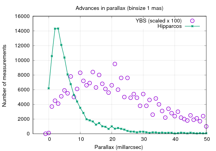
However, no such devices could make all-sky surveys. As a result, catalogs of stellar distances were incomplete, as well as being rather low in precision. For example, the Bright Star Catalog , compiled over the period of 1964 to 1991, listed parallax values for about 2700 stars.
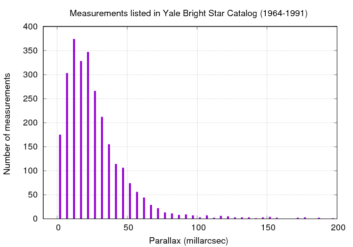
  Q:  What is the most common value for parallax (mas)?


  Q:  If we could measure stars perfectly, what should
            the most common value be?
The fact that this histogram turns over below 15 mas is a sign that the precision of the typical measurement is ... about 15 mas.
  Q:  If the uncertainty of a typical measurement is
            15 mas, how far away can a star be
            and still have a "good" distance?
It turns out that the nature of parallax measurements means that the connection between the error in the measurement and the error in the distance is not simple. There are a number of tricky aspects which can make the analysis of, say, the possible bias in some catalog, a complicated matter.
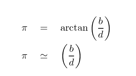
The first big problem is that the quantity of interest, the distance to a star d, is INVERSELY related to the measured angle π.
This means that an error of (for example) 20 percent in the measurement does NOT mean that there will be an error of 20 percent in the computed distance.
Why not? Well, let's do an example to find out. Suppose that we measure the parallax to a star to be
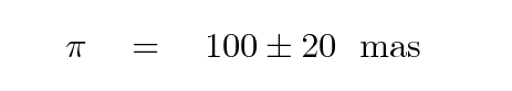
If the uncertainty is the usual "1-sigma" variety, then this measurement means that the true value of the parallax angle has a 66% chance of lying in the range 80 to 120 mas.
        angle < 80 mas                 16% probability

        80 mas < angle < 120 mas       66% probability

        120 mas < angle                16% probability
Fine so far. But what does that mean for distance we derive from this angle? We need to calculate the distance corresponding to the angle (100 - 20) and the angle (100 + 20). I'll let you fill in the table below.
                  distance <  ___ pc       16% probability

        ___ pc  < distance <  ___ pc       66% probability

        ___ pc  < distance                 16% probability

The fundamental issue here is that a realistic, symmetric error in the measured angle leads to an ASYMMETRIC error in the derived distance. The larger the fractional error in parallax angle becomes, the more asymmetric this error in the derived distance. For example, if we measure
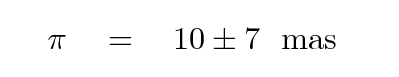
then the range of distances consistent with the measurement at 1-sigma looks like this:

We can sum up this first problem: symmetric errors in a measured parallax angle lead to asymmetric errors in the derived distance ... with a larger range of possible true distances on the "farther away" side.
The really nasty bit of the errors-in-parallax discussion is a consequence of the first conclusion: symmetric errors in angle lead to asymmetric errors in distance. Let's go back to this example again:
Based on the parallax angle π = 10 mas, we derive a distance of d = 100 pc --- but due to the uncertainty in the angle, the true location of the star has a 66% chance of lying anywhere within the range of 59 - 333 pc.
What that means is that the TRUE location of the star could be here ...
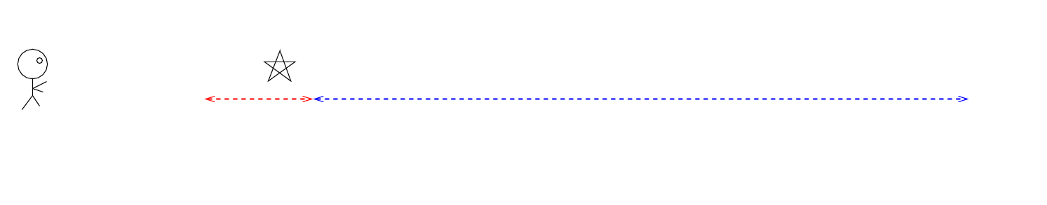
or here

or here

In fact, the star could lie anywhere along a line in this direction, with equal probability (*),
(*) Yes, yes, if the uncertainty has a gaussian distribution, then the probability that the error has any particular value is not uniform. Let's ignore that for simplicity's sake in the following discussion -- but one can NOT ignore it when doing proper statistical analysis.based on that one measurement. In a one-dimensional universe, the probability that the TRUE location of the star is farther than 100 pc is larger than the probability that the star is closer than 100 pc, simply by the ratio of the lengths of the possible locations:

    true location is closer      length  100 -  59  =   41 pc

    true location is farther     length  333 - 100 =   233 pc


    probability that star is farther than 100 pc      333 - 100
   ---------------------------------------------  =   ---------  ~  5.7
    probability that star is closer  than 100 pc      100 -  59
In a TWO-DIMENSIONAL universe, the probabilities would change because the region in which a "farther-than-100-pc" star could exist becomes much larger than that of a "closer-than-100-pc" star.

  Q:  What is the ratio of probabilities now?


    probability that star is farther than 100 pc
   ---------------------------------------------  =
    probability that star is closer  than 100 pc
Our course, our real universe is THREE-DIMENSIONAL. Sorry, I can't draw a good 3-D figure showing the two regions, but I hope you can extrapolate from the two-dimensional case to the three-dimensional one.
  Q:  What is the ratio of probabilities now, in 3-D?


    probability that star is farther than 100 pc
   ---------------------------------------------  =
    probability that star is closer  than 100 pc
Now, what's the big deal about all of this? The big deal is that we live in a region of relatively uniform stellar density. In our neighborhood of the Milky Way, there are roughly equal numbers of stars in all directions: left, right, up, down, forward, back. Yes, there tend to be more stars in the plane of the Milky Way, but the thickness of the disk is (until Gaia) larger than typical distance we could measure via parallax, that doesn't really matter.
And so, suppose that we measure the parallax to a star to have the value 10 +/- 1 mas, corresponding to a measured distance of 100 pc. There are three possibilities for the TRUE distance to this star:
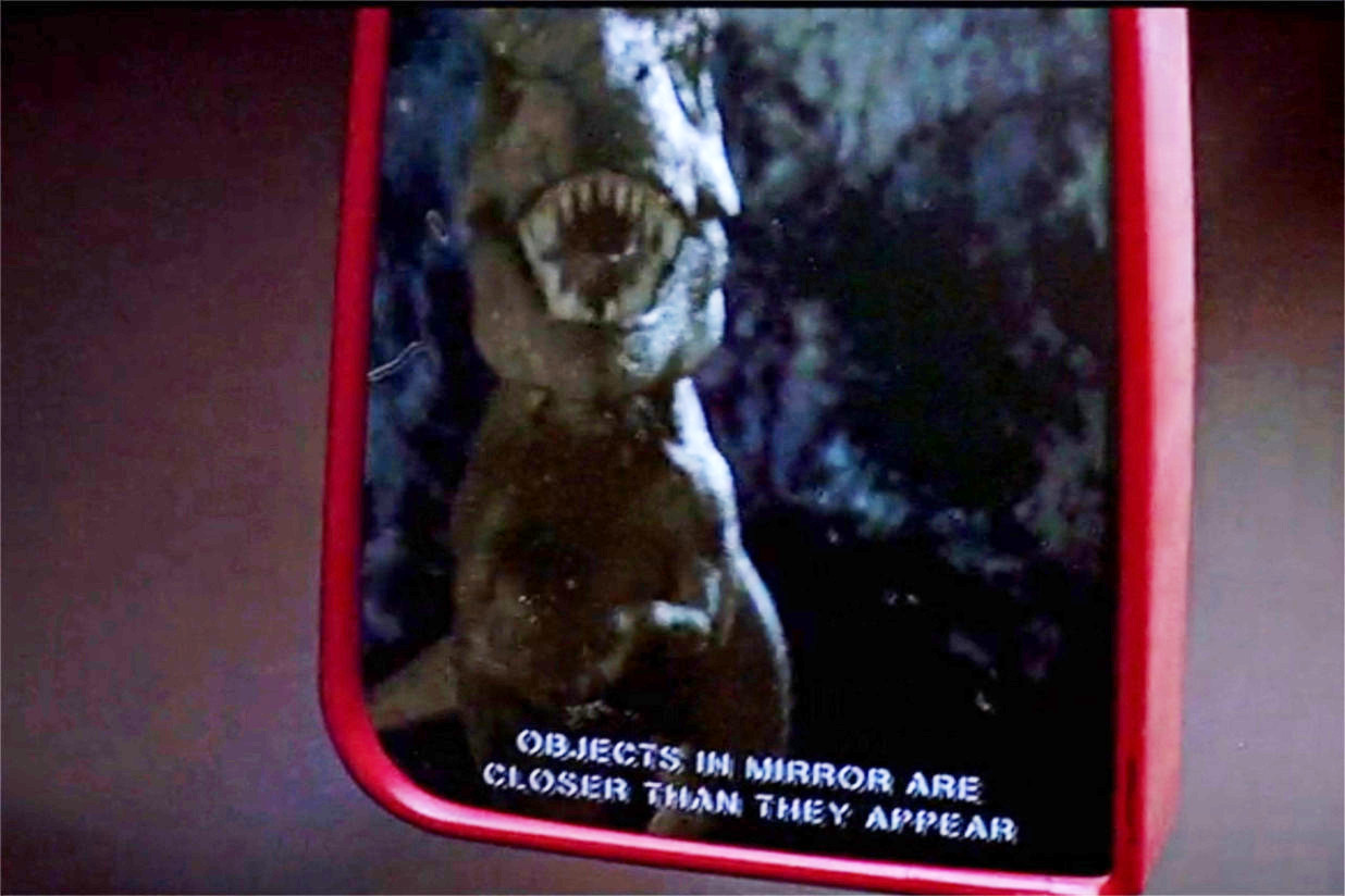
Which of these is most likely? The answer is "C". Because there are more stars in the "more distant" volume, it is more likely that a distant star has been improperly measured than a nearby star. The result is that our measurements of parallax lead to a systematic bias: stars appear closer than they really are (sort of like dinosaurs.)
This effect was noted long ago, by Trumpler and Weaver (1953), among others, but Lutz and Kelker first analyzed it detail in 1973. Astronomers sometimes refer to this bias, or the corrections needed to account for it, as the "Lutz-Kelker effect."
The size of this bias depends (mostly) on the ratio of the uncertainty in parallax to the value of parallax:

The inverse of this ratio, parallax divided by its uncertainty, is sometimes called "parallax_over_error." We'll see that version of the ratio near the end of today's class.
Let's look at some examples. We will observe a set of stars with measured parallax angles of exactly 10.0 mas, which means derived distances of exactly 100 pc.
When the fractional error is very small -- just a few percent -- then the errors in the derived distances, and the overall bias, are pretty small.

But as the fractional uncertainty grows, the errors and bias increase. Even uncertainties of just 10% can cause big mistakes in the measured parallax. Notice the long tail of true distances out to 140 pc and beyond; the errors in those derived distances are 40 percent or more, far larger than the 10% uncertainty in the parallax angle itself.

If the uncertainty becomes 20% or larger, the results involve errors which are frequently a factor of 2 or more. No one should try to use such measurements for any careful calculations.

Things are just silly when the uncertainty is 30%!

This table summarizes the results of a simulation in which I created a region of space with uniform stellar density, "measured" enough stars to find 1000 falling within a particular range of parallax values around 10 mas, and then compared those "measured" distances to the actual distances.
       Results of simulations with unform stellar density
           Stars with a measured parallax π = 10 mas
             and a measured distance of 100 pc

  uncertainty            actual distances (pc)
    σπ                mean       median      IQM        IQ range
   ------------------------------------------------------------------
   0.1  =  1%        100.04      100.09     100.06      0.78
   0.2     2%        100.33      100.30     100.27      1.55

   0.5     5%        101.60      101.27     101.29      3.87
   1.0    10%        106.95      105.26     105.57      8.95

   2.0    20%        162.8       143.3      146.9      39
   3.0    30%        626         662        645       221
   ------------------------------------------------------------------
The moral of this story is -- don't trust distances based on parallax unless the uncertainty in the measurement is much smaller than the measurement itself. I would prefer not to rely on any measurements in which the fractional uncertainty is larger than 10 percent.
The Hipparcos satellite was launched in 1989 and its first catalog was released in 1997. This project immediately improved our knowledge of stellar distances (and motions, and luminosities) by a large amount. Not only did it cover the entire sky, and measure stars fainter than those typically found in parallax catalogs (down to about mag 10), it also had a typical precision of about 2 mas. In other words, its typical measurement was about as good as the very best ground-based measurements.
  Q:  If the uncertainty of a typical measurement is
            2 mas, how far away can a star be
            and still have a "good" distance?
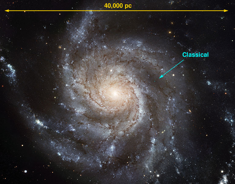
That's ... not a very large portion of our Milky Way Galaxy, as the figure below tries to indicate.
One of the wonderful results of Hippacos' measurements were the very accurate HR diagrams which could finally be made, since we now had LOTS of distance measurements to stars of all types. Below is one made using Hipparcos stars with uncertainties of ≤ 10% in their parallax angles.

Image courtesy of
ESA's page with HR diagrams based on Hipparcos data.
  Q:  How many different features can you identify
         on this HR diagram?
A sad note on the Gaia spacecraft (added Jan 14, 2025)
Gaia is a rather unusual "telescope," since it has been specially designed for astrometric observations. It resembles the Hipparcos satellite in many ways. The basic structure is built around two triple-mirror telescopes which point at regions in the sky separated by an angle of about 106.5 degrees.

Image courtesy of ESA/Atrium and
Spaceflight 101

Image courtesy of
Wikipedia
Light from the two telescopes is combined so that it falls upon the focal plane simultaneously. The telescope rotates with a period of six hours, causing stars to sweep across this focal plane in about 60 seconds. Objects in both directions are detected and measured together.
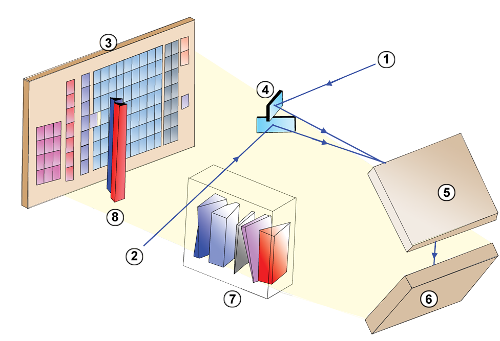
Image courtesy of
Wikipedia

Figure 1 from
Lindegren et al. 2016. Note that this figure
is rotated by 180 degrees relative to previous schematic.
The original caption follows.
Layout of the CCDs in Gaia's focal plane. Star images move from left to right in the diagram. As the images enter the field of view, they are detected by the sky mapper (SM) CCDs and astrometrically observed by the 62 CCDs in the astrometric field (AF). Basic-angle variations are interferometrically measured using the basic angle monitor (BAM) CCD in row 1 (bottom row in figure). The BAM CCD in row 2 is available for redundancy. Other CCDs are used for the red and blue photometers (BP, RP), radial velocity spectrometer (RVS), and wave- front sensors (WFS). The orientation of the field angles η (along-scan, AL) and ζ (across-scan, AC) is shown at bottom right. The actual origin (η, ζ) = (0, 0) is indicated by the numbered yellow circles 1 (for the preceding field of view) and 2 (for the following field of view).
The telescope slowly precesses, so that its spin sweeps out new areas in the sky over time. A typical star will be measured about 70 times over the course of the primary mission (2014 - 2019); that's about 14 measurements per year, though not all equally spaced.
Image courtesy of
Space Flight 101
As the spacecraft precesses, the "partners" of each star will gradually change. Eventually, the spacecraft will have many millions (billions?) of measurements of the relative positions of millions of stars. Scientists can then use a honking-big linear algebra procedure to solve simultaneously for the positions and motions of each star.
How precise are the measurements made by Gaia? The first results to be made public, as described in Lindegren et al. 2016, were called Gaia Data Release 1. This consisted of a limited set of measured properties for a very limited set of bright stars.
   Q:  What was the standard uncertainty in the
           parallax for a bright star in DR1?
           Look in Table 1 of  Lindegren et al. 2016

   Q:  Using that uncertainty, how far out into space
           could Gaia make good distance measurements as of 2017?
Even this first data release provided astronomers with many, many more stars than Hipparcos did, so it was possible to create much more detailed HR diagrams:

Image courtesy
ESA/Gaia/DPAC/IDT/FL/DPCE/AGIS
As time passed, and Gaia continued to scan the skies, it built up larger and larger sets of measurements of each star, allowing astronomers to create a better solution for the position, parallax, and proper motion of each object. Section 4 of the Gaia DR3 release documentation provides some measurements of the current (as of 2023) Gaia precision.

Part of Table 4.4 taken from
Section 4 of the Gaia DR3 release documentation
   Q:  What is the value for the standard uncertainty
           in the parallax of a brightish star?
           (Look in the figure above)

   Q:  Using that uncertainty, how far out into space
           will Gaia make good distance meausurements?
In any case, Gaia has greatly increased our knowledge of the stellar neighborhood. The DR3 release contains roughly 91 million stars with distances good to about 10 percent. The Hipparcos catalog contains only 0.12 million total entries, of which only about 0.04 million satisfy this criterion on quality.
As we will see in a future lecture, the star RR Lyrae is a very important one. It is one of the nearest and brightest of a class of pulsating stars which can help us to measure distances not only within the Milky Way, but to other galaxies.
Clearly, if we wish to use the class of RR Lyr stars as distance indicators, we need to know very precisely how luminous they are ... and, so, how far away they are. Let's consider the star RR Lyr itself.
This is, of course, just one star. But if our estimates of the distances to other stars, and other galaxies, depend upon RR Lyr stars in particular, and if the new Gaia data suggests that our old value might be incorrect by such an amount ... well, that should make you start to worry about the upper rungs on the Cosmological Distance Ladder!
As you know, the HR diagram provides a wealth of information about stellar properties.
HR diagram courtesy of
Richard Powell
The quantity shown on the vertical axis, absolute magnitude (or luminosity) depends critically on each star's distance.

That means that, if one tries to create an HR diagram from the measured properties of real stars (as opposed to some theoretical computed properties), one will be limited by the precision of one's knowledge of stellar distances. In practice, those distances are determined by parallax measurements. So, in a nutshell,
Let's practice grabbing data from the Gaia Archive, to see a bit of SQL in action, and then use the results to see how important the parallax measurement can be.
If one visits the Gaia Archive and chooses the "Search" button, one will be taken to a window which provides access to the gigantic Gaia database. If one then chooses the "Advanced (ADQL)" option, one can use SQL (Structured Query Language) to pick and choose information from the archive.
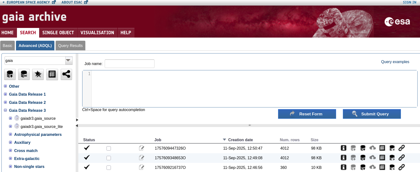
Here's an example of a query which chooses a small set of stars which have poor-quality measurements of parallax.
      select  parallax, phot_g_mean_mag, bp_rp,
            (phot_g_mean_mag + 5 - 5.0*LOG10(1000.0/parallax)) as abs_mag
      from gaiadr3.gaia_source_lite
      where
           (parallax > 5) and (parallax_over_error > 200) and
           (phot_g_mean_mag < 18.0) and
           (random_index between 30000000 and 40000000)
 ;
If one submits this request to the Gaia archive, it will think for a few seconds and then return a set of stars which satisfy the conditions. Here's a view of the first few entries:

Ta-da! One can save the result to one's computer, and then play with it as much as one likes.
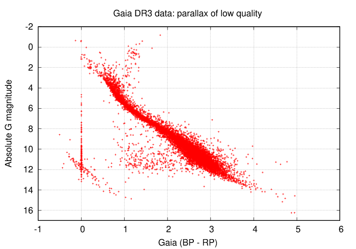
I've done this work for you. Below are two CSV datafiles, each with several thousand stars, based on queries like the one above. The difference between them is in the condition attached to each star's parallax_over_error value.
  low-quality           (parallax_over_error > 2)

  high-quality          (parallax_over_error > 200)
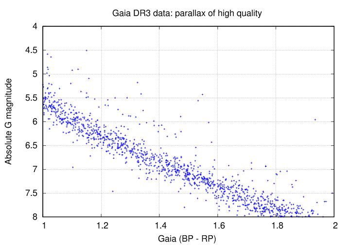
Please choose one datafile and create an HR diagram by plotting the color bp_rp on the horizontal axis, and abs_mag on the vertical axis.
Compare your graph with that of someone who chose the other option. What are the differences caused by the high-quality and low-quality parallax measurements?
In case we don't have time for the in-class exercise, we can look at these:
HR diagram based on low-quality parallax measurements
HR diagram based on high-quality parallax measurements
Do you see something interesting around the region where the color ranges between 1 and 2, and the absolute magnitude between 8 and 4?
Copyright © Michael Richmond.
This work is licensed under a Creative Commons License.


